Sam the Dog (see upper right-hand side of your screen) has passed on to a better place according to CNN. I can only hope that he's in a better place right now, cavorting with forty virgins in the fields of paradise.
sniff
In other news I have been catching up on my sleep since finishing my written thesis and all the bureaucracy associated with actually organizing my oral defense. Also Ben at theWatt.com has gone AWOL at the National Research Council labs so I have been trying to keep that site from becoming moribund. I promise to finish off some of the half-complete posts sitting in my box sometime soon. Of course, if my definition of soon is not the same as yours, too bad.
23 November 2005


13 November 2005
Embedded Energy Metric
Using thermodynamic laws it is usually fairly straightforward to analyze the efficiency of various systems of turning energy (more properly termed exergy) into work or heat. E.g. we can compare the ability of a heat pump next to electric resistance heaters to transform electricity into space heat. However it's often necessary to slide-slip away from the issue of the initial energy investment required to produce a baseboard heater compared to a heat pump because the data are proprietary or simply not gathered.
This energy investment in a product is known as the embedded energy. It is equivalent of capital investment in the money dimension. For example, in order to compare wind turbines to a combined-cycle thermal-electricity plant we should compare not only the CO2 offset by using wind rather than natural gas fuel to produce electricity but also the energy invested in the construction of the infrastructure as well. The steel and concrete in a wind turbine has an associated energy and CO2 production embedded into it during its manufacture. This embedded energy must be amortized over the lifespan of the turbine in order to properly determine the CO2 emissions that are offset.
The trick is how to determine the embedded energy in a product with adequate accuracy? To a certain extent this issue has stalled my investigation into the use of anerobic bioreactors to produce biogas from crop waste along with difficulties finding data on reaction rates as a function of temperature. Well, this being the blogosphere, an order of magnitude calculation on the back of an envelope should suffice. My thought is that if I could establish a metric for some common materials then I could simply estimate the embedded energy based on the mass of material in a product. The embedded energy problem is potentially simplified but it still remains challenging. Just try to find the mass of an air conditioner on a vendor's webpage, for example.
As a rough measure every material in the energy world can be subdivided into the following categories:
Rather than try to determine the energy embedded in a particular alloy I am hoping that StatsCan will have industry-wide figures for both production and energy consumption which will result in a more inclusive result. Hopefully I will be able to arrive at a reasonable set of metrics by the end of the week. Of course it would be desirable to actually check the results. Most likely there will be a need to introduce a fudge factor to account for the transformation of sheet steel into an automobile.
This energy investment in a product is known as the embedded energy. It is equivalent of capital investment in the money dimension. For example, in order to compare wind turbines to a combined-cycle thermal-electricity plant we should compare not only the CO2 offset by using wind rather than natural gas fuel to produce electricity but also the energy invested in the construction of the infrastructure as well. The steel and concrete in a wind turbine has an associated energy and CO2 production embedded into it during its manufacture. This embedded energy must be amortized over the lifespan of the turbine in order to properly determine the CO2 emissions that are offset.
The trick is how to determine the embedded energy in a product with adequate accuracy? To a certain extent this issue has stalled my investigation into the use of anerobic bioreactors to produce biogas from crop waste along with difficulties finding data on reaction rates as a function of temperature. Well, this being the blogosphere, an order of magnitude calculation on the back of an envelope should suffice. My thought is that if I could establish a metric for some common materials then I could simply estimate the embedded energy based on the mass of material in a product. The embedded energy problem is potentially simplified but it still remains challenging. Just try to find the mass of an air conditioner on a vendor's webpage, for example.
As a rough measure every material in the energy world can be subdivided into the following categories:
- Steel
- Aluminium
- Copper
- Plastic (polyethylene)
- Silicon
- Concrete
Rather than try to determine the energy embedded in a particular alloy I am hoping that StatsCan will have industry-wide figures for both production and energy consumption which will result in a more inclusive result. Hopefully I will be able to arrive at a reasonable set of metrics by the end of the week. Of course it would be desirable to actually check the results. Most likely there will be a need to introduce a fudge factor to account for the transformation of sheet steel into an automobile.
12 November 2005
Simple Solutions for Truck Freight Efficiency
I'm not one for "me-too" posts but it's been a couple of weeks now and I'm feeling the need to publish something. Green Car Congress carried a story about the development of a simple boat-tail attachment to a trailer that reduces the coefficient of drag of semi-tractor trailer vehicle by 0.12.
http://www.greencarcongress.com/2005/11/new_boat_tail_d.html
This just goes show how simple it could be to improve the efficiency of freight transport by truck. There's a number of other improvements that could be refited to existing truck fleets, like shrouding the tires and creating a flexible connector between the cab and trailer. Once it became clear that truck manufacturers weren't about to make improvements to the aerodynamics of their vehicles the government should have stepped in with legislation. Sometimes industries need a carrot to get them over a hill. In this case they need a kick in the ass to get them moving in the right direction.
http://www.greencarcongress.com/2005/11/new_boat_tail_d.html
This just goes show how simple it could be to improve the efficiency of freight transport by truck. There's a number of other improvements that could be refited to existing truck fleets, like shrouding the tires and creating a flexible connector between the cab and trailer. Once it became clear that truck manufacturers weren't about to make improvements to the aerodynamics of their vehicles the government should have stepped in with legislation. Sometimes industries need a carrot to get them over a hill. In this case they need a kick in the ass to get them moving in the right direction.
01 November 2005
Solar Thermal Cooling
Yes, I know it sounds like an oxymoron but just stick with me for a moment.
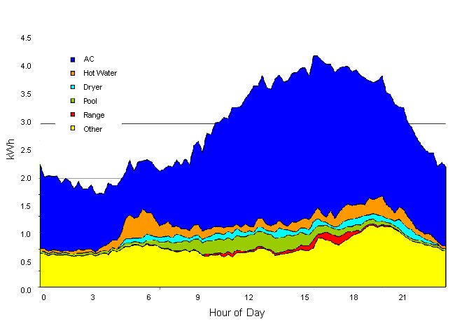
US peak electricity consumption occurs during the summer months when the demand for cooling is high and the efficiency of heat pumps drops with the higher ambient temperatures. Air conditioning constitutes approximately 15 % of annual US electricity consumption. However, the proportion of demand on peak days in hot states is in fact much higher.
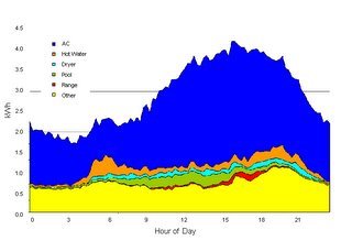
August day electrical consumption of a Florida home [Ref]
Supplying peak power is very expensive for utilities because they must build the infrastructure to cover peak demand which otherwise sits around underutilized. As a potential means of peak shaving we can examine the use of solar power to provide cooling. In this case utilities could be persuaded to offer businesses and home owners incentives to install such systems because it would improve their bottom line. The introduction of net metering with variable electricity prices could also provide an impetus. In the current environment of fixed rate electricity the consumer has little reason to purchase such a system.
There are two practical approaches:
A solar thermal system would use a collector to provide hot water for a single effect absorption chiller. Absorption chillers differ from common compression chillers in that cooling is driven by heat energy rather than mechanical energy. Aside from the plumping, several pieces of ancillary equipment are necessary including a controller, a pump, and a drain-back/expansion tank. Both systems are capable of providing hot water in addition to their cooling functions. For the PV system, a Heat Recovery Unit (HRU) would be used to pre-warm the water using waste heat from the heat pump.
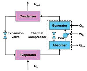
Some further explanation of absorption chillers is warranted given that they are relatively uncommon. An absorption chiller transfers thermal energy from the heat source to the heat sink through an absorbent fluid and a refrigerant. The absorption chiller accomplishes its refrigerative effect by absorbing and then releasing water vapor into and out of a lithium bromide or ammonia/water solution. The process begins as heat is applied at the generator and water vapor is driven off to a condenser. The cooled water vapor then passes through an expansion valve where the pressure reduces. The low-pressure water vapor then enters an evaporator, where ambient heat is added from a load and the actual cooling takes place. The heated, low-pressure vapor returns to the absorber, where it recombines with the lithium bromide and becomes a low-pressure liquid. This low-pressure solution is pumped to a higher pressure and into the generator to repeat the process.
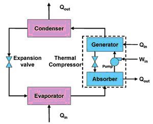
Schematic of Absorption Chiller Single-effect absorption chillers are not available for residential applications. Typically they are large units designed to operate off industrial waste heat. Small propane powered chillers are typically double-effect units that require a higher operating temperature than solar thermal collectors are capable of providing.
The performance of air conditioning systems is expressed by their coefficient of performance (COP). COP determines how many units of cooling/heating you get for every unit of energy you put in. Because units move heat the COP can be in excess of one. A typical value for a air conditioning heat pump is about 3.5 compared to only 0.7 for a absorption chiller.
The COP of an absorption chiller is heavily dependant on the applied temperature. If the solar thermal system is only capable of producing tepid water it will not function effectively. For my analysis I will assume that the absorption chiller requires an input temperature of 85 oC compared to the typically 55 - 60 oC required for residential hot water. The obvious conclusion from this is that the cheap unglazed flat-plate solar thermal systems used to warm pool water aren't going to provide the temperatures we need. Instead, we have to move up to evacuated tube collectors.
Evacuated tube solar thermal collectors are sold by companies such as www.apricus-solar.com. They incorporate a number of improvements to increase their efficiency and maximum operating temperature:
PV/Heat Pump: 0.125 * 3.5 = 0.44
Evacuated Solar-thermal/Absorption Chiller: 0.65 * 0.7 = 0.45
Amusingly they come out to being almost exactly the same. Assumably the inverter losses and parasitic heat losses are small and roughly equivalent. Presumably if you did an entropy analysis this would fall out quite naturally. Since the performance of each system is equivalent it is going to come down to cost.
If I size a 5000 W cooling system (for peak production at 1000 W/m2 insolation) for a home this is what I get:
This is ignoring mounts, plumbing and wiring for both the solar thermal collector and PV array. As we can see it is the cost of the evacuated solar collector pushing it above the PV solution. The expensive nature of evacuated solar thermal tubes is probably due to both their complexity and their low production volumes. Since they don't appear to be superior in this role now it seems unlikely that they would ever be able to catch up.
PV / Heat Pump System
Photovoltaic Panel
Name: Sharp ND-167U1
Peak Power: 167 W at 1000 W/m2 insolation
Module Efficiency 12.6 %
Area: 1.33 m
List Price: US$ 688.97
Heat Pump Chiller
Type: LG model LWK0710WGL
Cooling Power: 2051 W (7000 btu)
Coefficient of Performance: 3.43
Electrical Consumption: 600 W
List Price: US$ 330
Inverter
Type: Grid inter-tie
Name: Solectria PVI 1800W
Continuous Power Input Rating: 1980 W
Recommended Max PV Array Power: 2200 W
Continuous Power Output Rating: 1800 W
List Price: US$ 1731.25
Solar Thermal / Absorption Chiller System
Solar Collector
Name: Apricus 30 Tube Collector
Gathering Area: 2.4 m2
Estimated Peak Power Generation: 1536 W
Absorption Chiller
Name: Yakaza WFC-10
Cooling Power: 10 tons
Coefficient of Performance: 0.7
List Price: unknown (generally 2x that of heat pump)
Controller
Name: Apricus Sentinel-Pro controller
List Price: US $395
Pump
Name: Grundfos Stainless UP15-18SU
Power: 1/25 hp
List Price: $184
Drain-back/Expansion Tank
Name: Alternate Energy Technologies DB-10
Capacity: 10 gallons
List Price: $322
US peak electricity consumption occurs during the summer months when the demand for cooling is high and the efficiency of heat pumps drops with the higher ambient temperatures. Air conditioning constitutes approximately 15 % of annual US electricity consumption. However, the proportion of demand on peak days in hot states is in fact much higher.
Supplying peak power is very expensive for utilities because they must build the infrastructure to cover peak demand which otherwise sits around underutilized. As a potential means of peak shaving we can examine the use of solar power to provide cooling. In this case utilities could be persuaded to offer businesses and home owners incentives to install such systems because it would improve their bottom line. The introduction of net metering with variable electricity prices could also provide an impetus. In the current environment of fixed rate electricity the consumer has little reason to purchase such a system.
There are two practical approaches:
- Pair a photovoltaic array with a standard air conditioning unit.
- Pair a solar thermal collector with an aborption chiller.
A solar thermal system would use a collector to provide hot water for a single effect absorption chiller. Absorption chillers differ from common compression chillers in that cooling is driven by heat energy rather than mechanical energy. Aside from the plumping, several pieces of ancillary equipment are necessary including a controller, a pump, and a drain-back/expansion tank. Both systems are capable of providing hot water in addition to their cooling functions. For the PV system, a Heat Recovery Unit (HRU) would be used to pre-warm the water using waste heat from the heat pump.
Some further explanation of absorption chillers is warranted given that they are relatively uncommon. An absorption chiller transfers thermal energy from the heat source to the heat sink through an absorbent fluid and a refrigerant. The absorption chiller accomplishes its refrigerative effect by absorbing and then releasing water vapor into and out of a lithium bromide or ammonia/water solution. The process begins as heat is applied at the generator and water vapor is driven off to a condenser. The cooled water vapor then passes through an expansion valve where the pressure reduces. The low-pressure water vapor then enters an evaporator, where ambient heat is added from a load and the actual cooling takes place. The heated, low-pressure vapor returns to the absorber, where it recombines with the lithium bromide and becomes a low-pressure liquid. This low-pressure solution is pumped to a higher pressure and into the generator to repeat the process.
The performance of air conditioning systems is expressed by their coefficient of performance (COP). COP determines how many units of cooling/heating you get for every unit of energy you put in. Because units move heat the COP can be in excess of one. A typical value for a air conditioning heat pump is about 3.5 compared to only 0.7 for a absorption chiller.
The COP of an absorption chiller is heavily dependant on the applied temperature. If the solar thermal system is only capable of producing tepid water it will not function effectively. For my analysis I will assume that the absorption chiller requires an input temperature of 85 oC compared to the typically 55 - 60 oC required for residential hot water. The obvious conclusion from this is that the cheap unglazed flat-plate solar thermal systems used to warm pool water aren't going to provide the temperatures we need. Instead, we have to move up to evacuated tube collectors.
Evacuated tube solar thermal collectors are sold by companies such as www.apricus-solar.com. They incorporate a number of improvements to increase their efficiency and maximum operating temperature:
- The absorber is insulated from the air by a vacuum. This greatly decreases convective losses to the wind.
- The absorber is coating with a spectrally selective surface. Such a surface has a high absorption coefficient (α ~ 0.9 – 0.95) in the visible wavelengths (550 nm) but a low emissivity coefficient (ε ~ 0.02 – 0.08) in the far infra-red (10,000 nm). This reduces radiation losses to a minimum.
- Heat is transferred from the absorber to the working fluid by means of a heat pipe. A heat pipe is filled with a partial pressure of water, such that it boils at 30 °C. When the water evaporates, it convects up to a heat exchanger where it condenses, transferring its energy to the working fluid. The effective thermal conductance is roughly 10,000 times that of a solid copper bar. The heat pipe also has a diode function, in that if it is not hot enough to evaporate the water, no convection will occur.
PV/Heat Pump: 0.125 * 3.5 = 0.44
Evacuated Solar-thermal/Absorption Chiller: 0.65 * 0.7 = 0.45
Amusingly they come out to being almost exactly the same. Assumably the inverter losses and parasitic heat losses are small and roughly equivalent. Presumably if you did an entropy analysis this would fall out quite naturally. Since the performance of each system is equivalent it is going to come down to cost.
If I size a 5000 W cooling system (for peak production at 1000 W/m2 insolation) for a home this is what I get:
| Photovoltaic | Solar Thermal | ||
| Component | Normalized Cost (US$/Wcool) | Component | Normalized Cost (US$/Wcool) |
| PV Array | 1.21 | Solar Collector | 1.99 |
| Heat Pump | 0.16 | Absorption Chiller | 0.32 |
| Inverter | 0.34 | Pump | 0.037 |
| | Controller | 0.079 | |
| Drain-Back Tank | 0.064 | ||
| Total | 1.71 | Total | 2.49 |
This is ignoring mounts, plumbing and wiring for both the solar thermal collector and PV array. As we can see it is the cost of the evacuated solar collector pushing it above the PV solution. The expensive nature of evacuated solar thermal tubes is probably due to both their complexity and their low production volumes. Since they don't appear to be superior in this role now it seems unlikely that they would ever be able to catch up.
PV / Heat Pump System
Photovoltaic Panel
Name: Sharp ND-167U1
Peak Power: 167 W at 1000 W/m2 insolation
Module Efficiency 12.6 %
Area: 1.33 m
List Price: US$ 688.97
Heat Pump Chiller
Type: LG model LWK0710WGL
Cooling Power: 2051 W (7000 btu)
Coefficient of Performance: 3.43
Electrical Consumption: 600 W
List Price: US$ 330
Inverter
Type: Grid inter-tie
Name: Solectria PVI 1800W
Continuous Power Input Rating: 1980 W
Recommended Max PV Array Power: 2200 W
Continuous Power Output Rating: 1800 W
List Price: US$ 1731.25
Solar Thermal / Absorption Chiller System
Solar Collector
Name: Apricus 30 Tube Collector
Gathering Area: 2.4 m2
Estimated Peak Power Generation: 1536 W
Absorption Chiller
Name: Yakaza WFC-10
Cooling Power: 10 tons
Coefficient of Performance: 0.7
List Price: unknown (generally 2x that of heat pump)
Controller
Name: Apricus Sentinel-Pro controller
List Price: US $395
Pump
Name: Grundfos Stainless UP15-18SU
Power: 1/25 hp
List Price: $184
Drain-back/Expansion Tank
Name: Alternate Energy Technologies DB-10
Capacity: 10 gallons
List Price: $322
27 October 2005
Woohoo!
Let the record show that I finished my Master's thesis at 3:20 pm PST today. Of course I will still have to conduct revisions and defend it orally in a month but for all intents and purposes I've finished my first graduate degree. Now I have to start worrying about the Ph.D.
I am currently enjoying copious quantities of Hoegaarden beer so don't expect any intelligent commentary for tonight.
I am currently enjoying copious quantities of Hoegaarden beer so don't expect any intelligent commentary for tonight.
22 October 2005
A Quick Swipe at "Free" Hydrogen
I am busy with my thesis and marking at the moment but rather than issue corrections to my transport posts I just wanted to take a quick swipe at some specious hydrogen production claims.
A company called Alternate Energy Corporation claims to have some process that reacts water with metals to produce hydrogen gas. A quick browse of their website should set off alarm bells for anyone -- the distinct lack of any details on their system for example. Over at theWatt.com we've found some references to systems that burn aluminium to produce hydrogen. Aluminium won't react with water; you must introduce some acid or base to make the process run. Still, let's just imagine that we have the following irreversible reaction with zero enthalpy.
2 Al + 3H2O → Al2O3 + 3 H2
Given that you input 2 moles of Al for 6 moles of H it would require 9 kg of Aluminium to produce 1 kg of hydrogen. But the manufacture of aluminium is extremely energy intensive!!! Running the Aluminum Association's numbers I come up with 147.7 MJ/kg. This means you need 1329.3 MJ to produce one kilogram of hydrogen with an energy content of 142 MJ. This gives me an ERR of about 10 %. Whee.
If I ran a similarly fictitious reaction with iron I would need 18.6 kg of iron to make a kilogram of hydrogen. You can guess where this is going.
Now if we just burned the aluminium with oxygen in air... (we would have rocket fuel)
A company called Alternate Energy Corporation claims to have some process that reacts water with metals to produce hydrogen gas. A quick browse of their website should set off alarm bells for anyone -- the distinct lack of any details on their system for example. Over at theWatt.com we've found some references to systems that burn aluminium to produce hydrogen. Aluminium won't react with water; you must introduce some acid or base to make the process run. Still, let's just imagine that we have the following irreversible reaction with zero enthalpy.
2 Al + 3H2O → Al2O3 + 3 H2
Given that you input 2 moles of Al for 6 moles of H it would require 9 kg of Aluminium to produce 1 kg of hydrogen. But the manufacture of aluminium is extremely energy intensive!!! Running the Aluminum Association's numbers I come up with 147.7 MJ/kg. This means you need 1329.3 MJ to produce one kilogram of hydrogen with an energy content of 142 MJ. This gives me an ERR of about 10 %. Whee.
If I ran a similarly fictitious reaction with iron I would need 18.6 kg of iron to make a kilogram of hydrogen. You can guess where this is going.
Now if we just burned the aluminium with oxygen in air... (we would have rocket fuel)
20 October 2005
Hydrogen Debunked
Ulf Bossel, who is one of the leaders of the anti-hydrogen, pro-electricity and limited biomass lobby (of which I am a de facto member) has published a revised and more comprehensive version of his original 2003 study:
http://www.efcf.com/reports/E15.pdf
http://www.efcf.com/reports/E16.ppt
I made a PDF version of E16 for those of you without the latest version of Powerpoint.
http://www.efcf.com/reports/E15.pdf
http://www.efcf.com/reports/E16.ppt
I made a PDF version of E16 for those of you without the latest version of Powerpoint.
19 October 2005
A Candle that Burns Half as Bright Burns Twice as Long
My previous effort on the rolling and air resistance for trucking versus trains lends itself to an examination of dual-mode transportation. Dual mode systems typically allow a truck to run on rails in order to reduce the rolling resistance. An advanced and contemporary concept is the Bladerunner concept out of the UK. A mock-up of the concept can be viewed here.
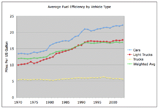
The trucking industry is one that has remained practically devoid of technological advances over the past thirty plus years. The fuel economy of transport trucks hasn't improved at all since 1980 (as far back as I have data). This is pretty surprising given that the cost of fuel is currently about twice the pay of the driver when driving at highway speeds. The mean pay for a trucker is $16.00/hr whereas a 5 mpg truck driving at 55 mph burns around $33.00 of diesel. I don't know what exactly to make of the lack of imagination.
I'll use the following assumptions for my hypothetical truck:
Loaded Mass: 35 000 kg
Frontal Area: 12 m2
Length: 15 m
Rolling Resistance Coefficient: 0.007
Rolling Resistance: 2400 N
Drag Coefficient: 0.7
Drag @ 110 km/h: 4500 N
Drag @ 80 km/h: 2400 N
The first and most obvious point of improvement is the aerodynamics. The drag coefficient for semi-tractor/trailers runs about 0.7 which is nowhere near the level obtained by modern automobiles (0.3). There's no real reason for trucks to be worse. In fact the Bladerunner concept shows a great deal of improvement in aerodynamics. They lowered the profile, improved the nose, eliminated the gap between the tractor and trailer, added aerodynamics to the wheels, and smoothed off all right angles.
Drag Coefficient: 0.3
Drag @ 110 km/h: 2000 N
Drag @ 80 km/h: 1000 N
This yields a pretty impressive drop from 6900 N overall resistance at 110 km/h to 4400 N which should result in a 55 % improvement in fuel economy. This can be achieved by cleaning up the aerodynamics of trucks to passenger car levels. I'm not taking into account the lower profile of the Bladerunner which would reduce the frontal area exposed to drag.
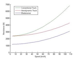
Fuel Economy of Truck Transport Systems
Now to examine the viability of running trucks on rails. The Bladerunner concept has a number of advantages by using the pneumatic tires as the power wheels and the steel bogies for load bearing. It breaks much faster and allows for much higher traffic density on the rail line. However this does come at a price. The rubber tires will no doubt impose their own rolling resistance. The Bladerunner article claims it halves the rolling resistance in exchange for 500 kg of extra mass for the rail bogies. This seems reasonable given that trains are about 3 - 6 times more efficient on the rolling resistance end. This would drop the rolling resistance from 2400 N to 1220 N. Practically speaking the extra mass of the bogies is irrelevant.
So if we compare our aerodynamic conventional truck to our aerodynamic Bladerunner the overall resistance is 4400 N and 3200 N respectively. The improvement in fuel economy is now 37.5 % which may be respectable enough to be economical. The full Bladerunner (3200 N) versus a contemporary (1970-tech) truck (6900 N) represents a fairly vast 115 % improvement. Cutting fuel consumption from truck shipping in half would represent a great reduction in the demand for petroleum.
Practically speaking in order to get the absolute best performance you would want Bladerunners to run in convoys so close together that they would be able to draft off each other. In this case the leading truck would have the hardest drive and the others would cut a break off his slipstream. Since this isn't exactly safe nor fair for the leading vehicle the obvious solution is to actually couple the vehicles in a convoy into a road/rail train. This would require a good communication system amongst the drivers if you wanted to be able to shift trucks in and out of a convoy on the move but it could certainly be worth it. If the vehicles were also hybrids driven by electrical motors then it would also be possible for the trailing vehicles to transfer power to the leading vehicle. In this case the following vehicles could completely retract their rubber wheels from the ground and travel solely on their steel bogies.
The other question to examine is how much is a driver's time worth? We can clearly see from the numbers that from a fuel economy perspective driving 30 km/h slower cuts the drag approximately in half. The disadvantage is that the driver must be paid more to drive more hours and the load will take a little longer to arrive. We can probably discount the amortization of the vehicle itself because that will be based on distance and not time traveled.
At a pay rate of $16.00/hr the marginal cost of slowing down 30 km/h is $6/hr or $0.075/km. With our current bad performance truck fleet slowing down by 30 km/h will shave off about 2100 N resistance, or 2.1 MJ/km. If we have a 30 % tank-to-wheel efficient engine (high side estimate) then we are reducing our burning of diesel by 7.0MJ/km. Diesel has an energy content of 46 MJ/kg and costs about $0.70/kg in the States. Hence our savings for traveling slower works out to $0.107/km. We're saving almost three cents a kilometer by driving slower. These numbers don't work out quite so well for the Bladerunner obviously. The efficiency gains will offset the economics to allow driving at a higher speed.
UPDATE: A quick check of my resistance numbers (6900 N at 30 % engine efficiency) show a burn rate of 23 MJ/km or half a kilogram of fuel. This works out to 4.3 mpg which is less than the fleet average of 5.3 mpg. This would be the case for driving in a straight line without any traffic or stops or hills etc. On the other hand, my truck is heavily loaded. The numbers seem reasonable to me although they could no doubt use some improvement.
Stuart Staniford at the Oil Drum put up a post about the fleet fuel economy numbers. I encourage readers in particular to look at the graph showing fuel economy for trucks. It's flat.
The trucking industry is one that has remained practically devoid of technological advances over the past thirty plus years. The fuel economy of transport trucks hasn't improved at all since 1980 (as far back as I have data). This is pretty surprising given that the cost of fuel is currently about twice the pay of the driver when driving at highway speeds. The mean pay for a trucker is $16.00/hr whereas a 5 mpg truck driving at 55 mph burns around $33.00 of diesel. I don't know what exactly to make of the lack of imagination.
I'll use the following assumptions for my hypothetical truck:
Loaded Mass: 35 000 kg
Frontal Area: 12 m2
Length: 15 m
Rolling Resistance Coefficient: 0.007
Rolling Resistance: 2400 N
Drag Coefficient: 0.7
Drag @ 110 km/h: 4500 N
Drag @ 80 km/h: 2400 N
The first and most obvious point of improvement is the aerodynamics. The drag coefficient for semi-tractor/trailers runs about 0.7 which is nowhere near the level obtained by modern automobiles (0.3). There's no real reason for trucks to be worse. In fact the Bladerunner concept shows a great deal of improvement in aerodynamics. They lowered the profile, improved the nose, eliminated the gap between the tractor and trailer, added aerodynamics to the wheels, and smoothed off all right angles.
Drag Coefficient: 0.3
Drag @ 110 km/h: 2000 N
Drag @ 80 km/h: 1000 N
This yields a pretty impressive drop from 6900 N overall resistance at 110 km/h to 4400 N which should result in a 55 % improvement in fuel economy. This can be achieved by cleaning up the aerodynamics of trucks to passenger car levels. I'm not taking into account the lower profile of the Bladerunner which would reduce the frontal area exposed to drag.

Now to examine the viability of running trucks on rails. The Bladerunner concept has a number of advantages by using the pneumatic tires as the power wheels and the steel bogies for load bearing. It breaks much faster and allows for much higher traffic density on the rail line. However this does come at a price. The rubber tires will no doubt impose their own rolling resistance. The Bladerunner article claims it halves the rolling resistance in exchange for 500 kg of extra mass for the rail bogies. This seems reasonable given that trains are about 3 - 6 times more efficient on the rolling resistance end. This would drop the rolling resistance from 2400 N to 1220 N. Practically speaking the extra mass of the bogies is irrelevant.
So if we compare our aerodynamic conventional truck to our aerodynamic Bladerunner the overall resistance is 4400 N and 3200 N respectively. The improvement in fuel economy is now 37.5 % which may be respectable enough to be economical. The full Bladerunner (3200 N) versus a contemporary (1970-tech) truck (6900 N) represents a fairly vast 115 % improvement. Cutting fuel consumption from truck shipping in half would represent a great reduction in the demand for petroleum.
Practically speaking in order to get the absolute best performance you would want Bladerunners to run in convoys so close together that they would be able to draft off each other. In this case the leading truck would have the hardest drive and the others would cut a break off his slipstream. Since this isn't exactly safe nor fair for the leading vehicle the obvious solution is to actually couple the vehicles in a convoy into a road/rail train. This would require a good communication system amongst the drivers if you wanted to be able to shift trucks in and out of a convoy on the move but it could certainly be worth it. If the vehicles were also hybrids driven by electrical motors then it would also be possible for the trailing vehicles to transfer power to the leading vehicle. In this case the following vehicles could completely retract their rubber wheels from the ground and travel solely on their steel bogies.
The other question to examine is how much is a driver's time worth? We can clearly see from the numbers that from a fuel economy perspective driving 30 km/h slower cuts the drag approximately in half. The disadvantage is that the driver must be paid more to drive more hours and the load will take a little longer to arrive. We can probably discount the amortization of the vehicle itself because that will be based on distance and not time traveled.
At a pay rate of $16.00/hr the marginal cost of slowing down 30 km/h is $6/hr or $0.075/km. With our current bad performance truck fleet slowing down by 30 km/h will shave off about 2100 N resistance, or 2.1 MJ/km. If we have a 30 % tank-to-wheel efficient engine (high side estimate) then we are reducing our burning of diesel by 7.0MJ/km. Diesel has an energy content of 46 MJ/kg and costs about $0.70/kg in the States. Hence our savings for traveling slower works out to $0.107/km. We're saving almost three cents a kilometer by driving slower. These numbers don't work out quite so well for the Bladerunner obviously. The efficiency gains will offset the economics to allow driving at a higher speed.
UPDATE: A quick check of my resistance numbers (6900 N at 30 % engine efficiency) show a burn rate of 23 MJ/km or half a kilogram of fuel. This works out to 4.3 mpg which is less than the fleet average of 5.3 mpg. This would be the case for driving in a straight line without any traffic or stops or hills etc. On the other hand, my truck is heavily loaded. The numbers seem reasonable to me although they could no doubt use some improvement.
Stuart Staniford at the Oil Drum put up a post about the fleet fuel economy numbers. I encourage readers in particular to look at the graph showing fuel economy for trucks. It's flat.
17 October 2005
Basic Bateria Flatulence
As dedicated readers of Entropy Production will know I am researching the potential to use the byproducts of biodiesel crops to produce biogas -- a mixture of methane and carbon dioxide -- and fertilizer sludge. I'm still coming up short on researching the engineering fudamentals of biological methane production. I would like to lay out the biological basics to form a framework for future analysis. Breaking up complex biological polymers into methane gas is a multi-step process involving many different populations of bacteria. Biology has the habit of splicing words together like German vocabulary; they call the process of methane production methanogensis.
There are two basic pathways. The first is the production of hydrogen directly from polymers. The second is a longer process that breaks down polymers to acetate. Methanogenesis can consume either CO2 and H2 or acetate ion (CH3CO2) which also produces CO2 as a byproduct. In addition to hydrogen and acetate some other fermentation products such as methanol can also be transformed into methane.
The acetate pathway is the longer of the two. The first step is the basic fermentation of proteins, fats, and carbohydrates into smaller chunks. The next step is to break down the intermediate products into acetate(CH3COO-) and acetic acid (CH3COOH). The pH of the solution can become unbalanced at this point which is disadvantageous to the consumption of acetane into methane.
The basic reaction is:
C2H4O2 → CH4 + CO2
The hydrogen pathway can consume most forms of biological material. It basic disadvantage is that the enzyme used rapidly reduces in effectiveness in the presence of hydrogen. The very production of hydrogen acts to stall the process. As such the hydrogen must be quickly removed from the system. Diffusion is generally slow but feeding the hydrogen into another chemical reaction can consume it quickly. Because the product is hydrogen gas there has been considerable research into this pathway. Research has focused on genetically modifying the enzyme to operate in the presence of hydrogen or engineering improvements to increase the yield. Methanogens (methane production bacteria) can react H2 with CO2 to form methane. This will produce oxygen gas which is not desirable in the anaerobic environment.
The basic reaction is:
CO2 + 2H2 → CH4 + O2
Methanogensis can only take place in an anaerobic environment. Maintaining an anaerobic environment not only protects the oxygen adverse bacteria but also prevents the growth of oxygen breathing methane burners.
The rate of methane production is highly dependant on pH and temperature. Most methanogens (mesophiles) prefer a temperature between 30 - 40 o and a pH near neutral (7.0) or slightly alkaline. My inability to find temperature and pH dependence is one of my stumbling points at the moment.
Methane producers are not the only bacteria in the pond that consume hydrogen and acetate. In particular, sulfur and nitrogen fixing bacteria both out compete methanogens for reactants. Sulfur fixing bacteria like to produce Hydrogen Sulfide gas (H2S) which then bubbles off and should be separated from the biogas flow. On the other hand, nitrogen fixing bacteria tend to produce ammonium ion (NH4+) which then finds something else to bond to. Ideally one might want to search for a bacterium that fixes sulfur into a solid form that is suitable for soil fertilization. Principally one could find data on the N and S content for Canola meal and figure the number of moles of H2 consumed.
Just as an aside, I did find some research on the production of butanol from biomass instead of ethanol. I don't have on-line access to this research so I can't easily review it but it is interesting nonetheless.
There are two basic pathways. The first is the production of hydrogen directly from polymers. The second is a longer process that breaks down polymers to acetate. Methanogenesis can consume either CO2 and H2 or acetate ion (CH3CO2) which also produces CO2 as a byproduct. In addition to hydrogen and acetate some other fermentation products such as methanol can also be transformed into methane.
The acetate pathway is the longer of the two. The first step is the basic fermentation of proteins, fats, and carbohydrates into smaller chunks. The next step is to break down the intermediate products into acetate(CH3COO-) and acetic acid (CH3COOH). The pH of the solution can become unbalanced at this point which is disadvantageous to the consumption of acetane into methane.
The basic reaction is:
C2H4O2 → CH4 + CO2
The hydrogen pathway can consume most forms of biological material. It basic disadvantage is that the enzyme used rapidly reduces in effectiveness in the presence of hydrogen. The very production of hydrogen acts to stall the process. As such the hydrogen must be quickly removed from the system. Diffusion is generally slow but feeding the hydrogen into another chemical reaction can consume it quickly. Because the product is hydrogen gas there has been considerable research into this pathway. Research has focused on genetically modifying the enzyme to operate in the presence of hydrogen or engineering improvements to increase the yield. Methanogens (methane production bacteria) can react H2 with CO2 to form methane. This will produce oxygen gas which is not desirable in the anaerobic environment.
The basic reaction is:
CO2 + 2H2 → CH4 + O2
Methanogensis can only take place in an anaerobic environment. Maintaining an anaerobic environment not only protects the oxygen adverse bacteria but also prevents the growth of oxygen breathing methane burners.
The rate of methane production is highly dependant on pH and temperature. Most methanogens (mesophiles) prefer a temperature between 30 - 40 o and a pH near neutral (7.0) or slightly alkaline. My inability to find temperature and pH dependence is one of my stumbling points at the moment.
Methane producers are not the only bacteria in the pond that consume hydrogen and acetate. In particular, sulfur and nitrogen fixing bacteria both out compete methanogens for reactants. Sulfur fixing bacteria like to produce Hydrogen Sulfide gas (H2S) which then bubbles off and should be separated from the biogas flow. On the other hand, nitrogen fixing bacteria tend to produce ammonium ion (NH4+) which then finds something else to bond to. Ideally one might want to search for a bacterium that fixes sulfur into a solid form that is suitable for soil fertilization. Principally one could find data on the N and S content for Canola meal and figure the number of moles of H2 consumed.
Just as an aside, I did find some research on the production of butanol from biomass instead of ethanol. I don't have on-line access to this research so I can't easily review it but it is interesting nonetheless.
16 October 2005
On The Rails
It's often stated that trains are far more efficient in transporting freight than semi-trucks. Trucks remain the primary freight movers however because of their versatility. By means of an electricity analogue, trains do transmission but trucks can perform both transmission and distribution services.
I thought it would be valuable to look at the major reasons why trains are more efficient than trucks. There are three main areas to look at:
Fd = 1/2 cdρAcv2
where Fd is the drag in Newtons, cd is the coefficient of drag, ρ is the density of air (1.17 kg/m3), Ac is the area cross-section, and v is the velocity in meters per second. For cargo transportation we should normalize the coefficient of drag by the ratio of the cross-sectional area to the overall length of the cargo carrier.
The rolling resistance on the other hand is not very dependant on speed. Drag is usually expressed as
Fr = crgm
where Fr is the rolling resistance in Newtons, cr is the coefficient of rolling resistance, g is the acceleration of gravity (9.81 m/s2) and m is the mass in kilograms.
Transient accelerations basically refers to traffic and hills. Trains have right of way so they don't have to stop and yield to other traffic at any time. Their rail lines also tend to go through or around hills rather than over them. As such they do not waste energy by speeding up or slowing down unnecessarily. Regenerative braking can mitigate this issue to a large extent.
Let's take a look at an example for a car, semi-truck, and a 50-car train.
Trucks are less aerodynamically efficient than cars for a variety of reasons: their blunt front-end, many exposed turning wheels, gap between the cab and trailer, and the sharp back end. I don't really know how aerodynamically efficient a train is but I can guess that it basically creates its own wind. On rolling resistance trucks have a minor advantage over cars because they operate at higher pneumatic pressure. The steel wheels on trains don't deform at all so they are considerably superior.
The key point is in fact the length to cross section area ratio and its impact on aerodynamic drag. If we normalize the coefficient of drag by the L:A ratio the results for cars and trucks are on the same order of magnitude, 0.6 and 0.2 respectively. The train normalized drag coefficient is dramatically lower at 0.01. Essentially because the front cars will push the wind the remaining cars get a free ride against air resistance. This reduces the overall air resistance on a train per unit mass of cargo regardless of its aerodynamic shape.
If we assume a mass of 35,000 kg for the semi and 2,500,000 kg for the train we can graph an estimate for the rolling and drag resistance:
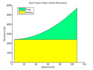
Semi-truck Resistance
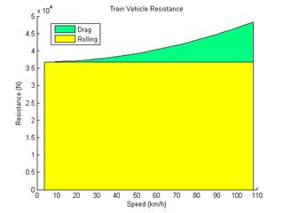
Train Resistance
The resistance at 108 km/h (30 m/s) works out to 0.16 N/kg for a truck and 0.02 N/kg for a train. In this estimate the train is about eight times more efficient. That matches well with generally quoted values. What's more significant is how the rolling resistance forms a much greater proportion of losses for the train compared to the truck. This underscores how the long length of the train gives it an advantage on the drag side of the equation.
I thought it would be valuable to look at the major reasons why trains are more efficient than trucks. There are three main areas to look at:
- Air drag
- Rolling resistance
- Transient accelerations
Fd = 1/2 cdρAcv2
where Fd is the drag in Newtons, cd is the coefficient of drag, ρ is the density of air (1.17 kg/m3), Ac is the area cross-section, and v is the velocity in meters per second. For cargo transportation we should normalize the coefficient of drag by the ratio of the cross-sectional area to the overall length of the cargo carrier.
The rolling resistance on the other hand is not very dependant on speed. Drag is usually expressed as
Fr = crgm
where Fr is the rolling resistance in Newtons, cr is the coefficient of rolling resistance, g is the acceleration of gravity (9.81 m/s2) and m is the mass in kilograms.
Transient accelerations basically refers to traffic and hills. Trains have right of way so they don't have to stop and yield to other traffic at any time. Their rail lines also tend to go through or around hills rather than over them. As such they do not waste energy by speeding up or slowing down unnecessarily. Regenerative braking can mitigate this issue to a large extent.
Let's take a look at an example for a car, semi-truck, and a 50-car train.
| Transport | Car | Semi | Train |
| cd | 0.3 | 0.7 | 2 |
| cr | 0.01 | 0.007 | 0.0015 |
| L:A ratio | 0.5/m | 3.5/m | 175/m |
Trucks are less aerodynamically efficient than cars for a variety of reasons: their blunt front-end, many exposed turning wheels, gap between the cab and trailer, and the sharp back end. I don't really know how aerodynamically efficient a train is but I can guess that it basically creates its own wind. On rolling resistance trucks have a minor advantage over cars because they operate at higher pneumatic pressure. The steel wheels on trains don't deform at all so they are considerably superior.
The key point is in fact the length to cross section area ratio and its impact on aerodynamic drag. If we normalize the coefficient of drag by the L:A ratio the results for cars and trucks are on the same order of magnitude, 0.6 and 0.2 respectively. The train normalized drag coefficient is dramatically lower at 0.01. Essentially because the front cars will push the wind the remaining cars get a free ride against air resistance. This reduces the overall air resistance on a train per unit mass of cargo regardless of its aerodynamic shape.
If we assume a mass of 35,000 kg for the semi and 2,500,000 kg for the train we can graph an estimate for the rolling and drag resistance:

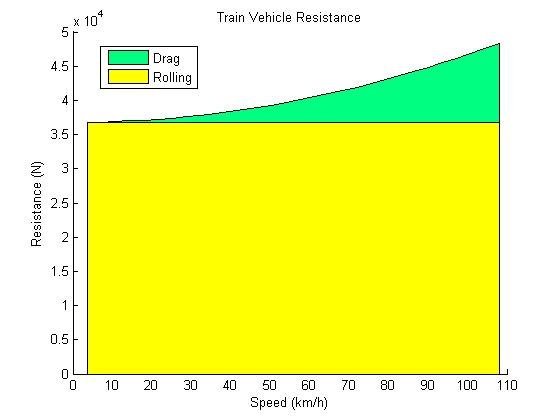
The resistance at 108 km/h (30 m/s) works out to 0.16 N/kg for a truck and 0.02 N/kg for a train. In this estimate the train is about eight times more efficient. That matches well with generally quoted values. What's more significant is how the rolling resistance forms a much greater proportion of losses for the train compared to the truck. This underscores how the long length of the train gives it an advantage on the drag side of the equation.
Subscribe to:
Posts (Atom)